1. Feedforward Neural Network Models

In this tutorial, we will learn how to use a neural network model to predict the energy of points on the Müller-Brown potential energy surface.

1.1. Defining the Müller-Brown Potential Energy Function

For the definition of Müller-Brown potential, see here.

\(v(x,y) = \sum_{k=0}^3 A_k \mathrm{exp}\left[ a_k (x - x_k^0)^2 + b_k (x - x_k^0) (y - y_k^0) + c_k (y - y_k^0)^2 \right] \)

from math import exp, pow

def mueller_brown_potential(x, y):
    A = [-200, -100, -170, 15]
    a = [-1, -1, -6.5, 0.7]
    b = [0, 0, 11, 0.6]
    c = [-10, -10, -6.5, 0.7]
    x0 = [1, 0, -0.5, -1.0]
    y0 = [0, 0.5, 1.5, 1]
    z = 0
    for k in range(4):
        # Scale the function by 0.1 to make plotting easier
        z += 0.1 * A[k] * exp(a[k] * pow(x-x0[k], 2) + b[k] * (x-x0[k]) * (y-y0[k]) + c[k] * pow(y-y0[k], 2))
    return z

1.1.1. Generate Training Data

First, we need to generate data to train the neural network.

import numpy as np

# generate x and y  on a grid
x_range = np.arange(-1.8, 1.4, 0.1, dtype=np.float32)
y_range = np.arange(-0.4, 2.4, 0.1, dtype=np.float32)
X, Y = np.meshgrid(x_range, y_range)

# compute the potential energy at each point on the grid
mueller_brown_potential_vectorized = np.vectorize(mueller_brown_potential, otypes=[np.float32])
Z = mueller_brown_potential_vectorized(X, Y)

# keep only low-energy points for training
train_mask = Z < 10
X_train, Y_train, Z_train = X[train_mask], Y[train_mask], Z[train_mask]

print(f"Z_min: {np.min(Z)}, Z_max: {np.max(Z)}")
print(f"Size of (future) training set: {len(Z_train)}")

Z_min: -14.599802017211914, Z_max: 1194.4622802734375
Size of (future) training set: 696

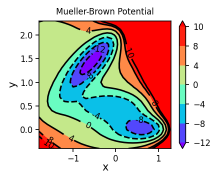
1.1.2. Visualizing Training Data: 3-D Projection Surface

We will now create a 3-D plot of our training data. We are going to use the plotly library to create an interactive plot. We only plot the part of the potential energy surface that is below 15 (arbitrary unit). For the actual training, only the part that is below 10 (arbitrary unit) will be used.

import plotly.graph_objects as go

fig = go.Figure(data=[go.Surface(z=Z, x=X, y=Y, colorscale='rainbow', cmin=-15, cmax=9)])
fig.update_traces(contours_z=dict(show=True, project_z=True))
fig.update_layout(title='Mueller-Brown Potential', width=500, height=500,
                  scene = dict(
                      zaxis = dict(dtick=3, range=[-15, 15]),
                      camera_eye = dict(x=-1.2, y=-1.2, z=1.2)))

1.1.3. Visualizing Training Data: Contour Surface

Now we will create a contour surface plot of our training data. Since we will plot similar contour surface plots later, we will define a function to do this.

import matplotlib.pyplot as plt

def plot_contour_map(X, Y, Z, ax, title, colorscale='rainbow', levels=None):
    if levels is None:
        levels = [-12, -8, -4, 0, 4, 8, 10]
    ct = ax.contour(X, Y, Z, levels, colors='k')
    ax.clabel(ct, inline=True, fmt='%3.0f', fontsize=8)
    ct = ax.contourf(X, Y, Z, levels, cmap=colorscale, extend='both', vmin=levels[0], vmax=levels[-1])
    ax.set_xlabel("x", labelpad=-0.75)
    ax.set_ylabel("y", labelpad=2.5)
    ax.tick_params(axis='both', pad=2, labelsize=8)
    cbar = plt.colorbar(ct)
    cbar.ax.tick_params(labelsize=8)
    ax.set_title(title, fontsize=8)


fig, ax = plt.subplots(figsize=(3, 2.5), dpi=150)
plot_contour_map(X, Y, Z, ax=ax, title='Mueller-Brown Potential')
fig.tight_layout()

1.2. Defining the Neural Network Class

1.2.1. A Basic Neural Network

Below is a schematic of a neural network. Inputs (\(x\), \(y\)) are given weights (\(w\)). For each neuron in the hidden layer a bias (\(b\)) is added to the weighted inputs to generate a value (\(v\)) for the activation function (tanh). The activation function decides the activity (\(v'\)) of each neuron in the hidden layer. Weights (\(w'\)), biases (\(b'\)), and the activation function on the neuron of the output layer produces the prediction (\(V^{pred}\)).

Here we define our neural network as a Python class. A function (\(\it{train\_loop}\)) is used to loop through our training data.

import torch
import torch.nn as nn
import torch.nn.functional as F

# Set default data type to float32
torch.set_default_dtype(torch.float32)


class NeuralNetwork(nn.Module):
    def __init__(self, n_hidden=20):
        """
        Args:
            n_hidden (int): Number of neurons in the hidden layer.
        """
        super().__init__()
        self.linear = nn.Sequential(
            nn.Linear(2, n_hidden), # Linear function taking 2 inputs and outputs data for n_hidden neurons.
            nn.Tanh(),
            nn.Linear(n_hidden, 1) # Linear function taking data from n_hidden neurons and producing one output value. 
        )

    def forward(self, x): 
        return self.linear(x)


def train_loop(dataloader, model, loss_fn, optimizer):
    model.train() # Set model to training mode.
    num_batches = len(dataloader)
    train_loss = 0
    for X, y in dataloader:
        # Compute prediction and loss
        pred = model(X)
        loss = loss_fn(pred.squeeze(), y)

        # Backpropagation - using the loss function gradients to update the weights and biases.
        optimizer.zero_grad() # Zero out the gradients from the previous iteration to replace them. 
        loss.backward() # Update the gradients of the loss function.
        optimizer.step() # Uses step() to optimize the weights and biases with the updated gradients. 

        with torch.no_grad():
            train_loss += loss.item()

    train_loss /= num_batches
    return train_loss

1.3. Loading PyTorch and Training Data

After installing and importing pytorch, we will save our training data as a tensor data set.

from torch.utils.data import TensorDataset, DataLoader

# turn NumPy arrays into PyTorch tensors
X_tensor = torch.from_numpy(np.column_stack((X_train, Y_train)))
Y_tensor = torch.from_numpy(Z_train)

dataset = TensorDataset(X_tensor, Y_tensor)
print(f"Size of training set: {len(dataset)}")

Size of training set: 696

1.4. Training the Model

Now we can train the neural network model. We will finish our training when the desired number of epochs has been reached. We will also define some terms used for training below.

Epochs - Number of forward/backward passes through the entire neural network.

Learning Rate - Determines the step size as we try to minimize the loss function. A faster learning rate would have a larger step size.

Stochastic Gradient Descent (SGD) - The algorithm used for minimizing the loss function.

Note: In this example, there are 696 training points broken into 87 batches of batch size 8.

# Set random seed for reproducibility
torch.manual_seed(314)

# Hyperparameters
batch_size = 32
epochs = 1000
learning_rate = 1e-2
n_hidden = 20

train_loader = DataLoader(dataset, batch_size=batch_size, shuffle=True)
model = NeuralNetwork(n_hidden)
loss_fn = nn.MSELoss()
optimizer = torch.optim.SGD(model.parameters(), lr=learning_rate)

print("Training Errors:")
for epoch in range(epochs):
    train_loss = train_loop(train_loader, model, loss_fn, optimizer)
    if (epoch + 1) % 100 == 0:
        print(f"epoch: {epoch:>3d}   loss: {train_loss:>6.3f}")
print("Done with Training!")

Training Errors:

epoch:  99   loss:  8.242

epoch: 199   loss:  2.019

epoch: 299   loss:  1.576

epoch: 399   loss:  1.281

epoch: 499   loss:  1.142

epoch: 599   loss:  0.992

epoch: 699   loss:  0.871

epoch: 799   loss:  0.842

epoch: 899   loss:  0.785

epoch: 999   loss:  0.745
Done with Training!

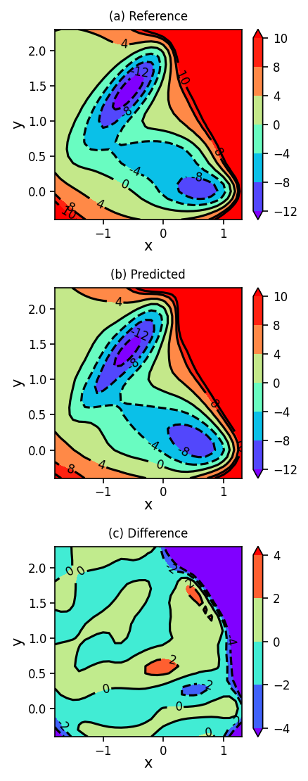
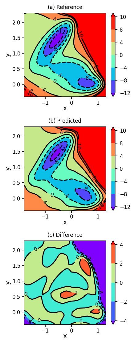
1.5. Plotting Reference, Predicted, and Difference Surfaces

Finally, we will plot the Müller-Brown potential energy surface using the analytical function (reference), using the neural network (predicted), and we will show the difference between the predicted and reference surfaces.

model.eval() # Set model to evaluation mode
Z_pred = model(torch.from_numpy(np.column_stack((X.flatten(), Y.flatten())))).detach().numpy().reshape(Z.shape)
Z_diff = Z_pred - Z

fig, ax = plt.subplots(3, figsize=(3, 7.5), dpi=150)
plot_contour_map(X, Y, Z, ax=ax[0], title='(a) Reference')
plot_contour_map(X, Y, Z_pred, ax=ax[1], title='(b) Predicted')
plot_contour_map(X, Y, Z_diff, ax=ax[2], title='(c) Difference', levels=[-4, -2, 0, 2, 4])
fig.tight_layout()

1.6. Taking a Look at the NN parameters

In order to take a closer look at the neural network parameters, we will plug them into the linear functions.

print("model:", model)

for name, param in model.named_parameters():
    if name == 'linear.0.weight': weights0 = param.data.detach().numpy()
    elif name == 'linear.0.bias': bias0 = param.data.detach().numpy()
    elif name == 'linear.2.weight': weights2 = param.data.detach().numpy()
    elif name == 'linear.2.bias': bias2 = param.data.detach().numpy()

xy0 = torch.tensor([-0.5, 1.5], dtype=torch.float32)
z0 = model(xy0)

#first linear function
v1 = np.zeros(n_hidden)
for i in range(n_hidden):
    v1[i] += weights0[i, 0] * xy0[0] + weights0[i, 1] * xy0[1] + bias0[i]

#activation function
v2 = np.zeros(n_hidden)
for i in range(n_hidden):
    v2[i] = np.tanh(v1[i])

#second linear function
z_pred = 0.0
for i in range(n_hidden):
    z_pred += weights2[0,i] * v2[i]
z_pred += bias2[0]

print("z0:", z0, "z_pred:", z_pred)

model: NeuralNetwork(
  (linear): Sequential(
    (0): Linear(in_features=2, out_features=20, bias=True)
    (1): Tanh()
    (2): Linear(in_features=20, out_features=1, bias=True)
  )
)
z0: tensor([-13.0163], grad_fn=<ViewBackward0>) z_pred: -13.016342414391445

1.7. A More Automated/Refined Implementation

1.7.1. A PyTorch-Lightning Implementation

Below is a more professional implementation of the neural network that saves epoch infromation in the logs_csv/ directory.

%pip install lightning --quiet
import lightning.pytorch as pl
from lightning.pytorch.loggers import CSVLogger

Note: you may need to restart the kernel to use updated packages.

class NeuralNetworkLightning(pl.LightningModule):
    def __init__(self, model, learning_rate):
        super().__init__()
        self.model = model
        self.learning_rate = learning_rate

    def forward(self, x):
        return self.model(x)

    def training_step(self, batch, batch_idx):
        x, y = batch
        y_pred = self.model(x)
        loss = F.mse_loss(y_pred.squeeze(), y)
        self.log('train_loss', loss)
        return loss

    def configure_optimizers(self):
        # Using the Adam optimzation algorithm instead of SGD. 
        optimizer = torch.optim.Adam(self.parameters(), lr=self.learning_rate)
        return [optimizer]

%%capture
# Set random seed for reproducibility
pl.seed_everything(314, workers=True);

# Hyperparameters
batch_size = 32
epochs = 1000
learning_rate = 1e-2
n_hidden = 20

train_loader = DataLoader(dataset, batch_size=batch_size, shuffle=True)
csv_logger = CSVLogger('logs_csv', version=0)
trainer = pl.Trainer(max_epochs=epochs, logger=csv_logger, deterministic=True)
model = NeuralNetworkLightning(NeuralNetwork(n_hidden), learning_rate)
trainer.fit(model, train_loader)

Seed set to 314

GPU available: False, used: False

TPU available: False, using: 0 TPU cores

IPU available: False, using: 0 IPUs

HPU available: False, using: 0 HPUs

  | Name  | Type          | Params
----------------------------------------
0 | model | NeuralNetwork | 81    
----------------------------------------
81        Trainable params
0         Non-trainable params
81        Total params
0.000     Total estimated model params size (MB)

`Trainer.fit` stopped: `max_epochs=1000` reached.

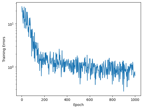
1.7.2. Plotting Training Error

Now we can plot the training error as the number of epochs increases.

import pandas as pd
loss = pd.read_csv("logs_csv/lightning_logs/version_0/metrics.csv")

fig, ax = plt.subplots()
ax.semilogy(loss["epoch"], loss["train_loss"])
ax.set_xlabel("Epoch")
ax.set_ylabel("Training Errors")

Text(0, 0.5, 'Training Errors')

1.7.3. Plotting Reference, Predicted, and Difference Surfaces

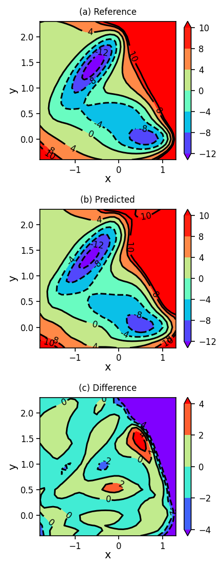
Again, we plot the reference, predicted, and difference surfaces using the more refined neural network implementation.

model.eval() # Set model to evaluation mode
Z_pred = model(torch.from_numpy(np.column_stack((X.flatten(), Y.flatten())))).detach().numpy().reshape(Z.shape)
Z_diff = Z_pred - Z

fig, ax = plt.subplots(3, figsize=(3, 7.5), dpi=150)
plot_contour_map(X, Y, Z, ax=ax[0], title='(a) Reference')
plot_contour_map(X, Y, Z_pred, ax=ax[1], title='(b) Predicted')
plot_contour_map(X, Y, Z_diff, ax=ax[2], title='(c) Difference', levels=[-4, -2, 0, 2, 4])
fig.tight_layout()

1.8. Train with Energy and Gradient

def mueller_brown_potential_gradient(x, y):
    A = [-200, -100, -170, 15]
    a = [-1, -1, -6.5, 0.7]
    b = [0, 0, 11, 0.6]
    c = [-10, -10, -6.5, 0.7]
    x0 = [1, 0, -0.5, -1.0]
    y0 = [0, 0.5, 1.5, 1]
    dx = 0
    dy = 0
    for k in range(4):
        dx += 0.1 * A[k] * exp(a[k] * pow(x-x0[k], 2) + b[k] * (x-x0[k]) * (y-y0[k]) + c[k] * pow(y-y0[k], 2)) * (a[k] * 2 *(x-x0[k]) + b[k] * (y-y0[k]))
        dy += 0.1 * A[k] * exp(a[k] * pow(x-x0[k], 2) + b[k] * (x-x0[k]) * (y-y0[k]) + c[k] * pow(y-y0[k], 2)) * (b[k] * (x-x0[k])+ c[k] * 2 * (y-y0[k]))
    return dx, dy

# compute the potential energy gradient at each point on the grid
mueller_brown_potential_gradient_vectorized = np.vectorize(mueller_brown_potential_gradient, otypes=[np.float32, np.float32])
dX, dY = mueller_brown_potential_gradient_vectorized(X, Y)

# keep only low-energy points for training
dX_train, dY_train = dX[train_mask], dY[train_mask]

dX_tensor = torch.from_numpy(np.column_stack((dX_train, dY_train)))
dataset = TensorDataset(X_tensor, Y_tensor, dX_tensor)

def train_loop_with_gradient(dataloader, model, loss_fn, optimizer):
    model.train() # Set model to training mode.
    num_batches = len(dataloader)
    train_loss = 0
    train_loss_energy = 0
    train_loss_gradient = 0
    for X, y, dX in dataloader:
        # Compute prediction and loss
        y_pred = model(X)
        dX_pred = torch.autograd.grad(y_pred, X, grad_outputs=torch.ones_like(y_pred), create_graph=True)[0]
        loss_energy = loss_fn(y_pred.squeeze(), y)
        loss_gradient = loss_fn(dX_pred.squeeze(), dX)
        loss = loss_energy + loss_gradient

        # Backpropagation - using the loss function gradients to update the weights and biases.
        optimizer.zero_grad() # Zero out the gradients from the previous iteration to replace them. 
        loss.backward() # Update the gradients of the loss function.
        optimizer.step() # Uses step() to optimize the weights and biases with the updated gradients. 

        with torch.no_grad():
            train_loss += loss.item()
            train_loss_energy += loss_energy.item()
            train_loss_gradient += loss_gradient.item()

    train_loss /= num_batches
    train_loss_energy /= num_batches
    train_loss_gradient /= num_batches
    return train_loss, train_loss_energy, train_loss_gradient

# Set random seed for reproducibility
torch.manual_seed(314)

# Hyperparameters
batch_size = 32
epochs = 1000
learning_rate = 1e-3
n_hidden = 20

train_loader = DataLoader(dataset, batch_size=batch_size, shuffle=True)
model = NeuralNetwork(n_hidden)
loss_fn = nn.MSELoss()
optimizer = torch.optim.SGD(model.parameters(), lr=learning_rate)

print("Training errors:")
for epoch in range(epochs):
    X_tensor.requires_grad_(True)
    train_loss, train_loss_energy, train_loss_gradient = train_loop_with_gradient(train_loader, model, loss_fn, optimizer)
    if (epoch + 1) % 100 == 0:
        print(f"epoch: {epoch:>3d}   loss: {train_loss:>6.3f}   energy loss: {train_loss_energy:>6.3f}   gradient loss: {train_loss_gradient:>6.3f}")
print("Done with Training!")

Training errors:

epoch:  99   loss: 155.851   energy loss: 10.925   gradient loss: 144.926

epoch: 199   loss: 75.487   energy loss:  4.643   gradient loss: 70.844

epoch: 299   loss: 31.353   energy loss:  1.031   gradient loss: 30.322

epoch: 399   loss: 27.340   energy loss:  0.847   gradient loss: 26.493

epoch: 499   loss: 25.616   energy loss:  0.818   gradient loss: 24.797

epoch: 599   loss: 24.661   energy loss:  0.823   gradient loss: 23.838

epoch: 699   loss: 23.933   energy loss:  0.844   gradient loss: 23.089

epoch: 799   loss: 23.246   energy loss:  0.827   gradient loss: 22.418

epoch: 899   loss: 22.167   energy loss:  0.756   gradient loss: 21.412

epoch: 999   loss: 21.067   energy loss:  0.692   gradient loss: 20.375
Done with Training!

model.eval() # Set model to evaluation mode
Z_pred = model(torch.from_numpy(np.column_stack((X.flatten(), Y.flatten())))).detach().numpy().reshape(Z.shape)
Z_diff = Z_pred - Z

fig, ax = plt.subplots(3, figsize=(3, 7.5), dpi=150)
plot_contour_map(X, Y, Z, ax=ax[0], title='(a) Reference')
plot_contour_map(X, Y, Z_pred, ax=ax[1], title='(b) Predicted')
plot_contour_map(X, Y, Z_diff, ax=ax[2], title='(c) Difference', levels=[-4, -2, 0, 2, 4])
fig.tight_layout()