![]()
5. Behler-Parrinello Fitting Neural Network with Machine Learning Potential (BP-FNN MLP) Models for the Claisen Rearrangement#
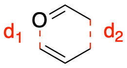
For this tutorial, we will be combining the Fitting Neural Network (FNN) from Lesson 1 and the Behler-Parrinello Neural Network (BPNN) from Lesson 3 to train a \(\Delta\) Machine Learning Potential (\(\Delta\)MLP) model to reproduce the energy and forces for the claisen rearrangement reaction. With a BP-FNN, we can utilize the symmetry functions from the BPNN model for feature extraction and use the FNN for training. The goal of this model is to train with data that is from the semiempirical (PM3) and DFT (B3LYP) levels of theory. The BP-FNN will be used to correct the semiempirical values to obtain DFT level accuracy, that makes it a \(\Delta\)MLP model. The reaction coordinate is constructed by stretching the \(d_2\) bond distance, while shrinking the \(d_1\) bond distance. The reaction is sampled with 21 windows along the \(d_1-d_2\) reaction coordinate.
Total of 2100 frames (1 ps/window) are saved every 1 fs.
from IPython.display import HTML

HTML(f"""<video src="https://github.com/cc-ats/mlp_tutorial/raw/main/Claisen_Rearrangement/img/claisen.mp4" width=300 controls/>""")
5.1. Importing PyTorch Lightning and Libraries#
We will first install PyTorch Lightning and import libraries needed to train our machine learning models.
%%capture
!pip install pytorch-lightning > /dev/null
import math
import numpy as np
from typing import Sequence, Tuple

import torch
import torch.nn as nn
import torch.nn.functional as F
from torch import Tensor

from torch.utils.data import TensorDataset, DataLoader, random_split
import pytorch_lightning as pl
from pytorch_lightning import loggers as pl_loggers
5.2. Defining Symmetry Functions#
We will define the BP and ANI symmetry functions to ensure that our ML predictions are invariant to translations, rotations, and permutations.
pairwise_vector: Distance function for calculating distances between each atom.
symmetry_function_g1: BP radial symmetry function.
symmetry_function_g2: BP angular symmetry function.
symmetry_function_g2ani: ANI angular symmetry function.
def pairwise_vector(coords: Tensor) -> Tensor:
    num_batches, num_channels, _ = coords.size()
    rij = coords[:, :, None] - coords[:, None]
    mask = ~torch.eye(num_channels, dtype=torch.bool, device=coords.device) # remove self-interaction
    rij = torch.masked_select(rij, mask.unsqueeze(2)).view(num_batches, num_channels, num_channels - 1, 3)
    return rij


def symmetry_function_g1(rij: Tensor, Rcr: float, EtaR: Tensor, ShfR: Tensor) -> Tensor:
    dij = torch.norm(rij, dim=3)
    fij = (torch.cos(dij / Rcr * math.pi) + 1) * 0.5 * (dij <= Rcr)
    g1 = torch.sum(torch.exp(-EtaR.unsqueeze(dim=1) * (dij.unsqueeze(dim=-1) - ShfR.unsqueeze(dim=1))**2) * fij.unsqueeze(dim=-1), dim=2)
    return g1


def symmetry_function_g2(rij: Tensor, Rca: float, Zeta: Tensor, EtaA: Tensor, LamA: Tensor) -> Tensor:
    c = torch.combinations(torch.arange(rij.size(2)), r=2)
    rij = rij[:, :, c]
    r12 = rij[:, :, :, 0]
    r13 = rij[:, :, :, 1]
    r23 = r12 - r13
    d12 = torch.norm(r12, dim=3)
    d13 = torch.norm(r13, dim=3)
    d23 = torch.norm(r23, dim=3)
    f12 = (torch.cos(d12 / Rca * math.pi) + 1) * 0.5
    f13 = (torch.cos(d13 / Rca * math.pi) + 1) * 0.5
    f23 = (torch.cos(d23 / Rca * math.pi) + 1) * 0.5
    cosine = torch.einsum('ijkl,ijkl->ijk', r12, r13) / (d12 * d13)

    g2 = torch.sum(2**(1 - Zeta.unsqueeze(dim=1)) * (1 + LamA.unsqueeze(dim=1) * cosine.unsqueeze(dim=-1))**Zeta.unsqueeze(dim=1) * torch.exp(-EtaA.unsqueeze(dim=1) * (d12**2 + d13**2 + d23**2).unsqueeze(dim=-1)) * (f12 * f13 * f23).unsqueeze(dim=-1), dim=2)
    return g2


def symmetry_function_g2ani(rij: Tensor, Rca: float, Zeta: Tensor, ShfZ: Tensor, EtaA: Tensor, ShfA: Tensor) -> Tensor:
    c = torch.combinations(torch.arange(rij.size(2)), r=2)
    rij = rij[:, :, c]
    r12 = rij[:, :, :, 0]
    r13 = rij[:, :, :, 1]
    r23 = r12 - r13
    d12 = torch.norm(r12, dim=3)
    d13 = torch.norm(r13, dim=3)
    f12 = (torch.cos(d12 / Rca * math.pi) + 1) * 0.5
    f13 = (torch.cos(d13 / Rca * math.pi) + 1) * 0.5
    cosine = torch.einsum('ijkl,ijkl->ijk', r12, r13) / (d12 * d13)
    cosine = torch.cos(torch.acos(cosine).unsqueeze(dim=-1) - ShfA.unsqueeze(dim=1))

    g2 = torch.sum(2**(1 - Zeta.unsqueeze(dim=1)) * (1 + cosine)**Zeta.unsqueeze(dim=1) * torch.exp(-EtaA.unsqueeze(dim=1) * (0.5 * (d12 + d13).unsqueeze(dim=-1) - ShfZ.unsqueeze(dim=1))**2) * (f12 * f13).unsqueeze(dim=-1), dim=2)
    return g2
5.3. Defining Neural Network and Feature Extraction Classes#
We will now define feature extraction classes which will be used in our Behler-Parrinello and ANI neural networks.
5.3.1. Defining Sequential and Dense Classes#
The Sequential class contains the function for the feed-forward aspect of our neural network. The Dense class contains functions to describe a densely connected neural network.
class Sequential(nn.Sequential):
    def forward(self, input: Tuple[Tensor, Tensor]) -> Tuple[Tensor, Tensor]:
        for module in self:
            input = module(input)
        return input

class Dense(nn.Module):
    def __init__(self, num_channels: int, in_features: int, out_features: int, bias: bool = True, activation: bool = False, residual: bool = False) -> None:
        super().__init__()
        self.num_channels = num_channels
        self.in_features = in_features
        self.out_features = out_features
        self.weight = nn.Parameter(torch.Tensor(num_channels, out_features, in_features))
        if bias:
            self.bias = nn.Parameter(torch.Tensor(num_channels, out_features))
        else:
            self.register_parameter('bias', None)
        self.activation = activation
        self.residual = residual
        self.reset_parameters()

    def reset_parameters(self) -> None:
        for w in self.weight:
            nn.init.kaiming_uniform_(w, a=math.sqrt(5))
        if self.bias is not None:
            for b, w in zip(self.bias, self.weight):
                fan_in, _ = nn.init._calculate_fan_in_and_fan_out(w)
                bound = 1 / math.sqrt(fan_in)
                nn.init.uniform_(b, -bound, bound)

    def forward(self, input: Tuple[Tensor, Tensor]) -> Tuple[Tensor, Tensor]:
        x, channels = input
        weight: Tensor = self.weight[channels]
        output: Tensor = torch.bmm(x.transpose(0, 1), weight.transpose(1, 2)).transpose(0, 1)

        if self.bias is not None:
            bias = self.bias[channels]
            output = output + bias

        if self.activation:
            output = torch.tanh(output)

        if self.residual:
            if output.shape[2] == x.shape[2]:
                output = output + x
            elif output.shape[2] == x.shape[2] * 2:
                output = output + torch.cat([x, x], dim=2)
            else:
                raise NotImplementedError("Not implemented")

        return output, channels

    def extra_repr(self) -> str:
        return 'num_channels={}, in_features={}, out_features={}, bias={}, activation={}, residual={}'.format(
            self.num_channels, self.in_features, self.out_features, self.bias is not None, self.activation, self.residual
        )
5.3.2. Defining the BP Feature Class#
Now we will create the feature class, which takes input information and uses functions to extract characteristics unique to the called input features. Here we will be using the previously defined symmetry functions for feature extraction.
class Feature(nn.Module):
    def __init__(self, Rcr: float, EtaR: Tensor, ShfR: Tensor, Rca: float, Zeta: Tensor, EtaA: Tensor, LamA: Tensor) -> None:
        super().__init__()
        assert len(EtaR) == len(ShfR) == len(LamA)
        assert len(Zeta) == len(EtaA)
        self.Rcr = Rcr
        self.Rca = Rca
        self.EtaR = torch.Tensor(EtaR)
        self.ShfR = torch.Tensor(ShfR)
        self.Zeta = torch.Tensor(Zeta)
        self.EtaA = torch.Tensor(EtaA)
        self.LamA = torch.Tensor(LamA)

    def forward(self, coords: Tensor, atom_types: Tensor) -> Tensor:
        num_batches, num_channels, _ = coords.size()
        rij = pairwise_vector(coords)
        EtaR = self.EtaR.to(device=coords.device)[atom_types]
        ShfR = self.ShfR.to(device=coords.device)[atom_types]
        Zeta = self.Zeta.to(device=coords.device)[atom_types]
        EtaA = self.EtaA.to(device=coords.device)[atom_types]
        LamA = self.LamA.to(device=coords.device)[atom_types]
        g1 = symmetry_function_g1(rij, self.Rcr, EtaR, ShfR)
        g2 = symmetry_function_g2(rij, self.Rca, Zeta, EtaA, LamA)

        return torch.concat((g1, g2), dim=2)

    @property
    def output_length(self) -> int:
        return len(self.EtaR[0]) + len(self.EtaA[0])
5.3.3. Defining the ANI Feature Class#
We will create a similar feature class for ANI that uses the ANI angle symmetry function.
class FeatureANI(nn.Module):
    def __init__(self, Rcr: float, EtaR: Tensor, ShfR: Tensor, Rca: float, Zeta: Tensor, ShfZ: Tensor, EtaA: Tensor, ShfA: Tensor) -> None:
        super().__init__()
        assert len(EtaR) == len(ShfR)
        assert len(Zeta) == len(ShfZ) == len(EtaA) == len(ShfA)
        self.Rcr = Rcr
        self.Rca = Rca
        self.EtaR = torch.Tensor(EtaR)
        self.ShfR = torch.Tensor(ShfR)
        self.Zeta = torch.Tensor(Zeta)
        self.ShfZ = torch.Tensor(ShfZ)
        self.EtaA = torch.Tensor(EtaA)
        self.ShfA = torch.Tensor(ShfA)

    def forward(self, coords: Tensor, atom_types: Tensor) -> Tensor:
        num_batches, num_channels, _ = coords.size()
        rij = pairwise_vector(coords)
        EtaR = self.EtaR.to(device=coords.device)[atom_types]
        ShfR = self.ShfR.to(device=coords.device)[atom_types]
        Zeta = self.Zeta.to(device=coords.device)[atom_types]
        ShfZ = self.ShfZ.to(device=coords.device)[atom_types]
        EtaA = self.EtaA.to(device=coords.device)[atom_types]
        ShfA = self.ShfA.to(device=coords.device)[atom_types]
        g1 = symmetry_function_g1(rij, self.Rcr, EtaR, ShfR)
        g2 = symmetry_function_g2ani(rij, self.Rca, Zeta, ShfZ, EtaA, ShfA)

        return torch.concat((g1, g2), dim=2)

    @property
    def output_length(self) -> int:
        return len(self.EtaR[0]) + len(self.EtaA[0])
5.3.4. Creating the Fitting Neural Network#
Now we create the Fitting class, which will use the dense neural network for fitting.
class Fitting(nn.Module):
    def __init__(self, n_types: int, in_features: int, neuron: Sequence[int] = [240, 240, 240]) -> None:
        super().__init__()
        layers = [Dense(n_types, in_features, neuron[0], activation=True)]
        for i in range(len(neuron)-1):
            layers.append(Dense(n_types, neuron[i], neuron[i+1], activation=True, residual=True))
        layers.append(Dense(n_types, neuron[-1], 1))
        self.fitting_net = Sequential(*layers)

    def forward(self, input : Tuple[Tensor, Tensor]) -> Tensor:
        output, _ = self.fitting_net(input)
        return output
5.3.5. The Behler-Parrinello Fitting Neural Network (BP-FNN)#
We create the BPNN class that can be used for feature extraction with the symmetry functions.
class BPNN(pl.LightningModule):
    def __init__(self, descriptor: nn.Module, fitting_net: nn.Module, learning_rate=5e-4) -> None:
        super().__init__()
        self.descriptor = descriptor
        self.fitting_net = fitting_net
        self.learning_rate = learning_rate

    def forward(self, coords: torch.Tensor, atom_types: torch.Tensor):
        coords.requires_grad_()
        descriptors = self.descriptor(coords, atom_types)
        atomic_energies = self.fitting_net((descriptors, atom_types))
        energy = torch.unbind(torch.sum(atomic_energies, dim=1))
        gradient, = torch.autograd.grad(energy, [coords], create_graph=True)
        return torch.hstack(energy), gradient

    def training_step(self, batch, batch_idx):
        qm_coord, atom_types, energy, gradient = batch
        ene_pred, grad_pred = self(qm_coord, atom_types[0])
        ene_loss = F.mse_loss(ene_pred, energy)
        grad_loss = F.mse_loss(grad_pred, gradient)

        lr = self.optimizers().optimizer.param_groups[0]['lr']
        start_lr = self.optimizers().optimizer.param_groups[0]['initial_lr']
        w_ene = 1
        w_grad = 1 + 99 * (lr / start_lr)

        loss = w_ene / (w_ene + w_grad) * ene_loss + w_grad / (w_ene + w_grad) * grad_loss
        self.log('train_loss', loss)
        self.log('l2_trn', torch.sqrt(loss))
        self.log('l2_e_trn', torch.sqrt(ene_loss))
        self.log('l2_f_trn', torch.sqrt(grad_loss))
        return loss

    def validation_step(self, batch, batch_idx):
        torch.set_grad_enabled(True)
        qm_coord, atom_types, energy, gradient = batch
        ene_pred, grad_pred = self(qm_coord, atom_types[0])
        ene_loss = F.mse_loss(ene_pred, energy)
        grad_loss = F.mse_loss(grad_pred, gradient)

        lr = self.optimizers().optimizer.param_groups[0]['lr']
        start_lr = self.optimizers().optimizer.param_groups[0]['initial_lr']
        w_ene = 1
        w_grad = 1 + 99 * (lr / start_lr)

        loss = w_ene / (w_ene + w_grad) * ene_loss + w_grad / (w_ene + w_grad) * grad_loss
        self.log('val_loss', loss)
        self.log('l2_tst', torch.sqrt(loss))
        self.log('l2_e_tst', torch.sqrt(ene_loss))
        self.log('l2_f_tst', torch.sqrt(grad_loss))
        self.log('lr', lr)
        return loss

    def configure_optimizers(self):
        optimizer = torch.optim.Adam(self.parameters(), lr=self.learning_rate)
        scheduler = {'scheduler': torch.optim.lr_scheduler.ExponentialLR(optimizer, 0.95),
                     'interval': 'epoch',
                     'frequency': 10,
                    }
        return [optimizer], [scheduler]
5.4. Importing Data and Seeding#
We will now import our semiempirical and DFT calculation data. We will then use seeding to generate random but reproducible training.
ds = np.DataSource(None)
qm_coord = np.array(np.load(ds.open("https://github.com/cc-ats/mlp_tutorial/raw/main/Claisen_Rearrangement/qm_coord.npy", "rb")), dtype="float32")
atom_types = np.loadtxt(ds.open("https://github.com/cc-ats/mlp_tutorial/raw/main/Claisen_Rearrangement/qm_elem.txt", "r"), dtype=int)
elems = np.unique(atom_types).tolist()
atom_types = np.array([[elems.index(i) for i in atom_types]])
atom_types = atom_types.repeat(len(qm_coord), axis=0)

energy = np.array((np.load(ds.open("https://github.com/cc-ats/mlp_tutorial/raw/main/Claisen_Rearrangement/energy.npy", "rb")) - np.load(ds.open("https://github.com/cc-ats/mlp_tutorial/raw/main/Claisen_Rearrangement/energy_sqm.npy", "rb"))) * 27.2114 * 23.061, dtype="float32")
energy = energy - energy.mean()
qm_gradient = np.array((np.load(ds.open("https://github.com/cc-ats/mlp_tutorial/raw/main/Claisen_Rearrangement/qm_grad.npy", "rb")) - np.load(ds.open("https://github.com/cc-ats/mlp_tutorial/raw/main/Claisen_Rearrangement/qm_grad_sqm.npy", "rb"))) * 27.2114 * 23.061 / 0.529177249, dtype="float32")

device = torch.device('cuda' if torch.cuda.is_available() else 'cpu')

qm_coord = torch.from_numpy(qm_coord).to(device)
atom_types = torch.from_numpy(atom_types).to(device)
energy = torch.from_numpy(energy).to(device)
qm_gradient = torch.from_numpy(qm_gradient).to(device)
pl.seed_everything(2)
dataset = TensorDataset(qm_coord, atom_types, energy, qm_gradient)
train, val = random_split(dataset, [2016, 84])
# Training Set Size: 2016 (96%)
# Test Set Size:       84 ( 4%)
# Data Set Size:     2100
train_loader = DataLoader(train, batch_size=32)
val_loader = DataLoader(val, batch_size=32)
INFO:lightning_fabric.utilities.seed:Global seed set to 2
5.5. Using ANI for Feature Extraction#
Here we set the parameters for the ANI model and begin training our BP-FNN.
%%capture
%%time
pl.seed_everything(2)

ani = True

if ani:
  # From TorchANI
  Rcr = 5.2000e+00
  Rca = 3.5000e+00
  EtaR = [1.6000000e+01]
  ShfR = [9.0000000e-01,1.1687500e+00,1.4375000e+00,1.7062500e+00,1.9750000e+00,2.2437500e+00,2.5125000e+00,2.7812500e+00,3.0500000e+00,3.3187500e+00,3.5875000e+00,3.8562500e+00,4.1250000e+00,4.3937500e+00,4.6625000e+00,4.9312500e+00]
  Zeta = [3.2000000e+01]
  ShfZ = [1.9634954e-01,5.8904862e-01,9.8174770e-01,1.3744468e+00,1.7671459e+00,2.1598449e+00,2.5525440e+00,2.9452431e+00]
  EtaA = [8.0000000e+00]
  ShfA = [9.0000000e-01,1.5500000e+00,2.2000000e+00,2.8500000e+00]
  EtaR, ShfR = np.array(np.meshgrid(EtaR, ShfR)).reshape(2, -1)
  Zeta, ShfZ, EtaA, ShfA = np.array(np.meshgrid(Zeta, ShfZ, EtaA, ShfA)).reshape(4, -1)
  EtaR = np.repeat([EtaR], 3, axis=0)
  ShfR = np.repeat([ShfR], 3, axis=0)
  Zeta = np.repeat([Zeta], 3, axis=0)
  ShfZ = np.repeat([ShfZ], 3, axis=0)
  EtaA = np.repeat([EtaA], 3, axis=0)
  ShfA = np.repeat([ShfA], 3, axis=0)
  descriptor = FeatureANI(Rcr, EtaR, ShfR, Rca, Zeta, ShfZ, EtaA, ShfA)
else:
  Rcr = 6.0
  Rca = 6.0
  ShfR = np.zeros((3,6)) # H, C, O
  EtaR = [0.0, 0.04, 0.14, 0.32, 0.71, 1.79]
  EtaR = np.repeat([EtaR], 3, axis=0) # H, C, O
  Zeta = [1, 2, 4, 8, 16, 32, 1, 2, 4, 8, 16, 32]
  Zeta = np.repeat([Zeta], 3, axis=0) # H, C, O
  EtaA = [0.0, 0.04, 0.14, 0.32, 0.71, 1.79, 0.0, 0.04, 0.14, 0.32, 0.71, 1.79]
  EtaA = np.repeat([EtaA], 3, axis=0) # H, C, O
  LamA = [1, 1, 1, 1, 1, 1, -1, -1, -1, -1, -1, -1]
  LamA = np.repeat([LamA], 3, axis=0) # H, C, O
  descriptor = Feature(Rcr, EtaR, ShfR, Rca, Zeta, EtaA, LamA)

fitting_net = Fitting(3, descriptor.output_length, neuron=[240, 240, 240])
model = BPNN(descriptor, fitting_net, learning_rate=5e-4)
csv_logger = pl_loggers.CSVLogger('logs_csv/')
trainer = pl.Trainer(max_epochs=100, logger=csv_logger, log_every_n_steps=20, accelerator='auto')
trainer.fit(model, train_loader, val_loader)
model.to(device)
INFO:lightning_fabric.utilities.seed:Global seed set to 2
INFO:pytorch_lightning.utilities.rank_zero:GPU available: True (cuda), used: True
INFO:pytorch_lightning.utilities.rank_zero:TPU available: False, using: 0 TPU cores
INFO:pytorch_lightning.utilities.rank_zero:IPU available: False, using: 0 IPUs
INFO:pytorch_lightning.utilities.rank_zero:HPU available: False, using: 0 HPUs
INFO:pytorch_lightning.accelerators.cuda:LOCAL_RANK: 0 - CUDA_VISIBLE_DEVICES: [0]
INFO:pytorch_lightning.callbacks.model_summary:
  | Name        | Type       | Params
-------------------------------------------
0 | descriptor  | FeatureANI | 0
1 | fitting_net | Fitting    | 383 K
-------------------------------------------
383 K     Trainable params
0         Non-trainable params
383 K     Total params
1.532     Total estimated model params size (MB)
INFO:pytorch_lightning.utilities.rank_zero:`Trainer.fit` stopped: `max_epochs=100` reached.
5.6. Saving the Model with PyTorch Files and Evaluating the Model’s Accuracy Using RMSD#
5.6.1. Saving the Model with PyTorch#
The following files are saved:
1) model.pt
torch.save saves tensors to model.pt
2) model_script.pt
torch.jit.save attempts to preserve the behavior of some operators across PyTorch versions.
Previously saved models can be loaded with:
model.load_state_dict(torch.load(”model.pt”))
torch.jit.load(“model_script.pt”)
torch.save(model.state_dict(), 'model.pt')
torch.jit.save(model.to_torchscript(), "model_script.pt")
ene_pred, grad_pred = model(qm_coord, atom_types[0])
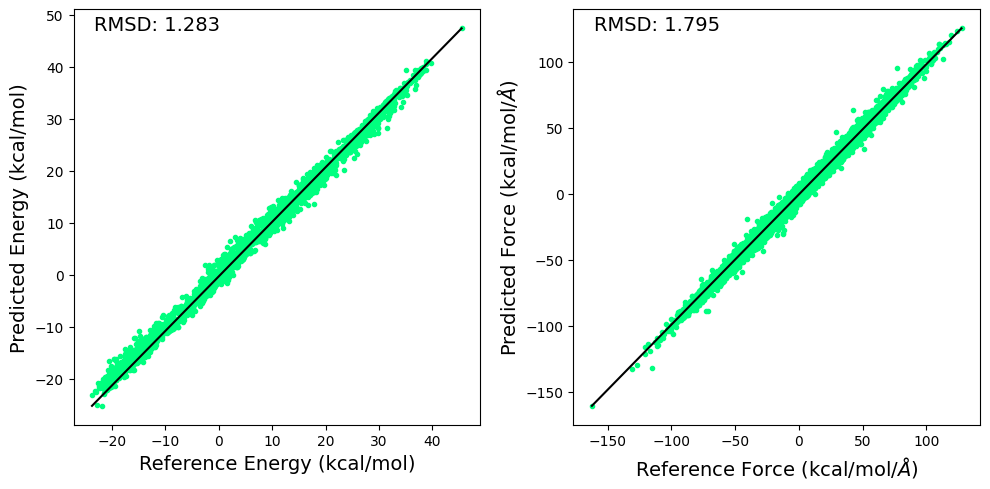
5.6.2. Plotting RMSD for \(\Delta\)MLP Energy and Forces#
RMSD for predicted and reference energy and forces are calculated and displayed below.
import matplotlib.pyplot as plt

fig, ax = plt.subplots(1,2,figsize=(10,5))

e1 = energy.cpu().detach().numpy() + np.load(ds.open("https://github.com/cc-ats/mlp_tutorial/raw/main/Claisen_Rearrangement/energy_sqm.npy","rb")) * 27.2114 * 23.061
e2 = ene_pred.cpu().detach().numpy() + np.load(ds.open("https://github.com/cc-ats/mlp_tutorial/raw/main/Claisen_Rearrangement/energy_sqm.npy","rb")) * 27.2114 * 23.061

ax[0].plot(e1, e2, linestyle='none', marker='.', color='springgreen')
ax[0].plot([np.max(e1), np.min(e1)], [np.max(e2), np.min(e2)] , color="k", linewidth=1.5)
ax[0].set_xlabel("Reference Energy (kcal/mol)", size=14)
ax[0].set_ylabel("Predicted Energy (kcal/mol)", size=14)
ax[0].annotate('RMSD: %.3f' % np.sqrt(np.mean((e1 - e2)**2)), xy=(0.05, 0.95), xycoords='axes fraction', size=14)

f1 = -qm_gradient.cpu().detach().numpy().reshape(-1) - np.load(ds.open("https://github.com/cc-ats/mlp_tutorial/raw/main/Claisen_Rearrangement/qm_grad_sqm.npy","rb")).reshape(-1) * 27.2114 * 23.061 / 0.529177249
f2 = -grad_pred.cpu().detach().numpy().reshape(-1) - np.load(ds.open("https://github.com/cc-ats/mlp_tutorial/raw/main/Claisen_Rearrangement/qm_grad_sqm.npy","rb")).reshape(-1) * 27.2114 * 23.061 / 0.529177249

ax[1].plot(f1, f2, linestyle='none', marker='.', color='springgreen')
ax[1].plot([np.max(f1), np.min(f1)], [np.max(f2), np.min(f2)] , color="k", linewidth=1.5)
ax[1].set_xlabel(r'Reference Force (kcal/mol/$\AA$)', size=14)
ax[1].set_ylabel(r'Predicted Force (kcal/mol/$\AA$)', size=14)
ax[1].annotate('RMSD: %.3f' % np.sqrt(np.mean((f1 - f2)**2)), xy=(0.05, 0.95), xycoords='axes fraction', size=14)

plt.tight_layout()
plt.savefig('rmsd.png', dpi=300)
5.6.3. The Model Weights and Biases Dictionary#
This cell prints the size of the weights and biases used in the trained model for reference.
print("Model's state_dict:")
for param_tensor in model.state_dict():
    print(param_tensor, "\t", model.state_dict()[param_tensor].size())
Model's state_dict:
fitting_net.fitting_net.0.weight 	 torch.Size([3, 240, 48])
fitting_net.fitting_net.0.bias 	 torch.Size([3, 240])
fitting_net.fitting_net.1.weight 	 torch.Size([3, 240, 240])
fitting_net.fitting_net.1.bias 	 torch.Size([3, 240])
fitting_net.fitting_net.2.weight 	 torch.Size([3, 240, 240])
fitting_net.fitting_net.2.bias 	 torch.Size([3, 240])
fitting_net.fitting_net.3.weight 	 torch.Size([3, 1, 240])
fitting_net.fitting_net.3.bias 	 torch.Size([3, 1])
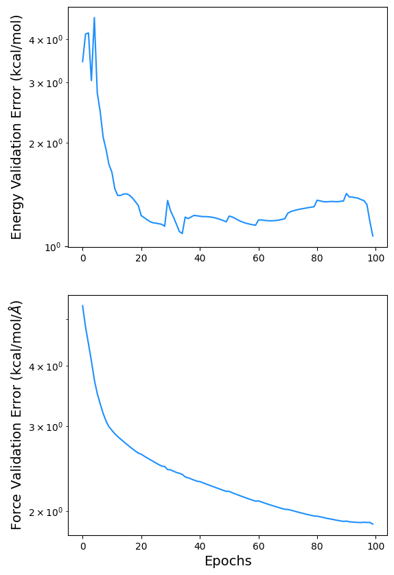
5.7. Plotting the Minimization of the Loss Function#
5.7.1. Plotting Validation Error for \(\Delta\)MLP#
Validation error for the \(\Delta\)MLP is shown below.
import pandas as pd

data = pd.read_csv(f'logs_csv/lightning_logs/version_{csv_logger.version}/metrics.csv')
fig, ax = plt.subplots(2, figsize=(6,10))
x = data['epoch'][~data['l2_e_tst'].isnull()]
y = data['l2_e_tst'][~data['l2_e_tst'].isnull()]
y2 = data['l2_f_tst'][~data['l2_f_tst'].isnull()]
ax[0].semilogy(x, y,color='dodgerblue')
ax[0].set_ylabel('Energy Validation Error (kcal/mol)',size=14)
ax[1].semilogy(x, y2, label='Force Validation Error (kcal/mol',color='dodgerblue')
ax[1].set_xlabel('Epochs',size=14)
ax[1].set_ylabel(r'Force Validation Error (kcal/mol/$\AA$)',size=14)
fig.savefig('loss.png', dpi=300)
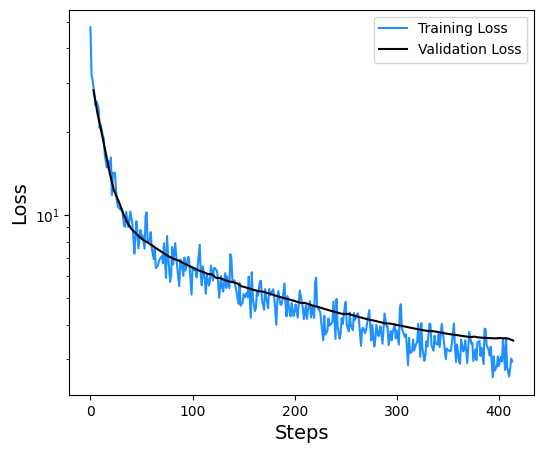
5.7.2. Plotting Training and Validation Loss for \(\Delta\)MLP#
The loss at each step of the training process is displayed below.
data = pd.read_csv(f'logs_csv/lightning_logs/version_{csv_logger.version}/metrics.csv')
fig, ax = plt.subplots(figsize=(6,5))
x = data['epoch'][~data['epoch'].isnull()]
y = data['train_loss'][~data['train_loss'].isnull()]
print(len(y))
plt.semilogy(y, label='Training Loss',color='dodgerblue')
y = data['val_loss'][~data['val_loss'].isnull()]
print(len(y))
plt.semilogy(y, label='Validation Loss',color='k')
plt.xlabel('Steps',size=14)
plt.ylabel('Loss',size=14)
plt.legend()
315
100
<matplotlib.legend.Legend at 0x7cc48e7a5870>